flowchart LR
subgraph Developer["👨💻 Developer"]
PUSH["git push"]
PR["Open PR"]
end
subgraph GitHub["⚙️ GitHub"]
ACTIONS["GitHub Actions"]
WORKFLOWS[".github/workflows/"]
end
subgraph Display["📊 Display Methods"]
COMMENT["💬 PR Comments
• Quick preview
• Stats
• Code blocks"] ARTIFACT["📦 Artifacts
• Full download
• All files
• Reports"] PAGES["🌐 GitHub Pages
• API docs
• Website
• Landing page"] LIVE["🚀 Live Preview
• Vercel
• Netlify
• Dashboard"] end subgraph Output["📄 HTML Output"] INDEX["index.html"] DOCS["API Documentation"] COVERAGE["Coverage Reports"] BENCH["Benchmark Results"] DASHBOARD["Performance Dashboard"] end PUSH --> ACTIONS PR --> ACTIONS ACTIONS --> WORKFLOWS WORKFLOWS --> Display COMMENT --> INDEX COMMENT --> STATS["Stats & Badges"] ARTIFACT --> COVERAGE ARTIFACT --> BENCH PAGES --> DOCS PAGES --> INDEX LIVE --> DASHBOARD LIVE --> UI["UI Preview"] style Developer fill:#e1f5fe,stroke:#01579b,stroke-width:2px style GitHub fill:#f3e5f5,stroke:#4a148c,stroke-width:2px style Display fill:#fff3e0,stroke:#e65100,stroke-width:2px style Output fill:#e8f5e9,stroke:#1b5e20,stroke-width:2px
• Quick preview
• Stats
• Code blocks"] ARTIFACT["📦 Artifacts
• Full download
• All files
• Reports"] PAGES["🌐 GitHub Pages
• API docs
• Website
• Landing page"] LIVE["🚀 Live Preview
• Vercel
• Netlify
• Dashboard"] end subgraph Output["📄 HTML Output"] INDEX["index.html"] DOCS["API Documentation"] COVERAGE["Coverage Reports"] BENCH["Benchmark Results"] DASHBOARD["Performance Dashboard"] end PUSH --> ACTIONS PR --> ACTIONS ACTIONS --> WORKFLOWS WORKFLOWS --> Display COMMENT --> INDEX COMMENT --> STATS["Stats & Badges"] ARTIFACT --> COVERAGE ARTIFACT --> BENCH PAGES --> DOCS PAGES --> INDEX LIVE --> DASHBOARD LIVE --> UI["UI Preview"] style Developer fill:#e1f5fe,stroke:#01579b,stroke-width:2px style GitHub fill:#f3e5f5,stroke:#4a148c,stroke-width:2px style Display fill:#fff3e0,stroke:#e65100,stroke-width:2px style Output fill:#e8f5e9,stroke:#1b5e20,stroke-width:2px
flowchart TD
subgraph Input["📥 Input"]
CODE["Source Code"]
HTML["HTML Files"]
RUST["Rust Code"]
end
subgraph Build["🔨 Build Stage"]
COMPILE["cargo build"]
DOC["cargo doc"]
BENCH["cargo bench"]
TEST["cargo test"]
end
subgraph Generate["📊 Generate HTML"]
COVERAGE[Coverage Report
cargo tarpaulin] DOCS[API Documentation
cargo doc] PERF[Performance Report
cargo bench] CUSTOM[Custom HTML
docs/ directory] end subgraph Workflows["⚙️ GitHub Workflows"] CI["CI.yml
- Build
- Test
- Lint"] DOCS_DEPLOY["Deploy Docs
- Build docs
- Deploy to Pages"] COV_DEPLOY["Coverage
- Generate
- Upload"] PREVIEW["Preview
- Deploy to Vercel
- Comment PR"] end subgraph Display["📺 Display Methods"] PR_COMMENT["💬 PR Comment
Summary + Stats"] ARTIFACTS["📦 Artifacts
Full Reports"] PAGES["🌐 GitHub Pages
API Documentation"] LIVE["🚀 Live Preview
Vercel/Netlify"] end CODE --> COMPILE HTML --> CUSTOM RUST --> COMPILE COMPILE --> TEST COMPILE --> BENCH COMPILE --> DOC TEST --> COVERAGE DOC --> DOCS BENCH --> PERF COVERAGE --> COV_DEPLOY DOCS --> DOCS_DEPLOY CUSTOM --> PREVIEW PERF --> CI COV_DEPLOY --> ARTIFACTS COV_DEPLOY --> PR_COMMENT DOCS_DEPLOY --> PAGES PREVIEW --> LIVE PREVIEW --> PR_COMMENT CI --> ARTIFACTS CI --> PR_COMMENT PR_COMMENT --> USER["👨💻 Developer"] ARTIFACTS --> USER PAGES --> USER LIVE --> USER style Input fill:#e1f5fe,stroke:#01579b,stroke-width:2px style Build fill:#f3e5f5,stroke:#4a148c,stroke-width:2px style Generate fill:#fff3e0,stroke:#e65100,stroke-width:2px style Workflows fill:#e8f5e9,stroke:#1b5e20,stroke-width:2px style Display fill:#fce4ec,stroke:#b71c1c,stroke-width:2px style USER fill:#fff9c4,stroke:#f57f17,stroke-width:2px
cargo tarpaulin] DOCS[API Documentation
cargo doc] PERF[Performance Report
cargo bench] CUSTOM[Custom HTML
docs/ directory] end subgraph Workflows["⚙️ GitHub Workflows"] CI["CI.yml
- Build
- Test
- Lint"] DOCS_DEPLOY["Deploy Docs
- Build docs
- Deploy to Pages"] COV_DEPLOY["Coverage
- Generate
- Upload"] PREVIEW["Preview
- Deploy to Vercel
- Comment PR"] end subgraph Display["📺 Display Methods"] PR_COMMENT["💬 PR Comment
Summary + Stats"] ARTIFACTS["📦 Artifacts
Full Reports"] PAGES["🌐 GitHub Pages
API Documentation"] LIVE["🚀 Live Preview
Vercel/Netlify"] end CODE --> COMPILE HTML --> CUSTOM RUST --> COMPILE COMPILE --> TEST COMPILE --> BENCH COMPILE --> DOC TEST --> COVERAGE DOC --> DOCS BENCH --> PERF COVERAGE --> COV_DEPLOY DOCS --> DOCS_DEPLOY CUSTOM --> PREVIEW PERF --> CI COV_DEPLOY --> ARTIFACTS COV_DEPLOY --> PR_COMMENT DOCS_DEPLOY --> PAGES PREVIEW --> LIVE PREVIEW --> PR_COMMENT CI --> ARTIFACTS CI --> PR_COMMENT PR_COMMENT --> USER["👨💻 Developer"] ARTIFACTS --> USER PAGES --> USER LIVE --> USER style Input fill:#e1f5fe,stroke:#01579b,stroke-width:2px style Build fill:#f3e5f5,stroke:#4a148c,stroke-width:2px style Generate fill:#fff3e0,stroke:#e65100,stroke-width:2px style Workflows fill:#e8f5e9,stroke:#1b5e20,stroke-width:2px style Display fill:#fce4ec,stroke:#b71c1c,stroke-width:2px style USER fill:#fff9c4,stroke:#f57f17,stroke-width:2px
graph LR
subgraph "Current State"
CPU_E["CPU"]
Copper["Copper Traces"]
Memory["Memory"]
CPU_E --- Copper
Copper --- Memory
end
subgraph "Transition Phase"
CPU_EIC["CPU"]
EIC["EIC Chiplet"]
Copper_Opt["Hybrid
Copper/ Optical"] Memory_Opt["Memory"] CPU_EIC --- EIC EIC --- Copper_Opt Copper_Opt --- Memory_Opt end subgraph "Future State" CPU_Opt["CPU"] EIC_Opt["EIC Chiplet"] Fiber["Optical Fiber"] Memory_Opt2["Optical Memory"] CPU_Opt --- EIC_Opt EIC_Opt --- Fiber Fiber --- Memory_Opt2 end CPU_E --> CPU_EIC Copper --> Copper_Opt Memory --> Memory_Opt CPU_EIC --> CPU_Opt Copper_Opt --> Fiber Memory_Opt --> Memory_Opt2 classDef current fill:#ffcdd2,stroke:#c62828,stroke-width:2px classDef transition fill:#fff9c4,stroke:#f57f17,stroke-width:2px classDef future fill:#c8e6c9,stroke:#2e7d32,stroke-width:2px class CPU_E,Copper,Memory current class CPU_EIC,EIC,Copper_Opt,Memory_Opt transition class CPU_Opt,EIC_Opt,Fiber,Memory_Opt2 future
Copper/ Optical"] Memory_Opt["Memory"] CPU_EIC --- EIC EIC --- Copper_Opt Copper_Opt --- Memory_Opt end subgraph "Future State" CPU_Opt["CPU"] EIC_Opt["EIC Chiplet"] Fiber["Optical Fiber"] Memory_Opt2["Optical Memory"] CPU_Opt --- EIC_Opt EIC_Opt --- Fiber Fiber --- Memory_Opt2 end CPU_E --> CPU_EIC Copper --> Copper_Opt Memory --> Memory_Opt CPU_EIC --> CPU_Opt Copper_Opt --> Fiber Memory_Opt --> Memory_Opt2 classDef current fill:#ffcdd2,stroke:#c62828,stroke-width:2px classDef transition fill:#fff9c4,stroke:#f57f17,stroke-width:2px classDef future fill:#c8e6c9,stroke:#2e7d32,stroke-width:2px class CPU_E,Copper,Memory current class CPU_EIC,EIC,Copper_Opt,Memory_Opt transition class CPU_Opt,EIC_Opt,Fiber,Memory_Opt2 future
flowchart LR
subgraph A [SOC / Chiplet 1]
direction LR
Core1[CPU Core]
Core2[CPU Core]
Mem1[Memory]
AXIBridge[AXI-to-UCIe
Offload Engine] Core1 --- Mem1 Core2 --- Mem1 Core1 --- AXIBridge Core2 --- AXIBridge end subgraph B [Chiplet 2] direction LR AXIBridge2[AXI-to-UCIe
Offload Engine] Accel[Accelerator] Mem2[Memory] Accel --- Mem2 Accel --- AXIBridge2 end AXIBridge ---|UCIe Interconnect| AXIBridge2
Offload Engine] Core1 --- Mem1 Core2 --- Mem1 Core1 --- AXIBridge Core2 --- AXIBridge end subgraph B [Chiplet 2] direction LR AXIBridge2[AXI-to-UCIe
Offload Engine] Accel[Accelerator] Mem2[Memory] Accel --- Mem2 Accel --- AXIBridge2 end AXIBridge ---|UCIe Interconnect| AXIBridge2
graph TB
subgraph "HIL Verification Platform"
subgraph "Host System"
H1[MATLAB/Simulink
Test Case Generation] H2[Python Scripts
Automation & Analysis] H3[UVM Testbench
Verification Environment] end subgraph "Real-Time Target Machine" R1[PLECS RT Box / Speedgoat
Real-Time Simulator] R2[Analog I/O
ADC/DAC 16-bit, 2Msps] R3[Digital I/O
PWM/GPIO 3.3V/5V] R4[Communication
SPI/I2C/CAN/UART] end subgraph "Device Under Test" D1[FPGA/SoC
DUT Hardware] D2[Analog Front-End
Sensors/Actuators] D3[Digital Core
CPU/MCU] D4[Mixed-Signal
ADC/DAC/PLL] end end %% Connections H1 -->|"Test Vectors"| R1 H2 -->|"Automation"| R1 H3 -->|"Verification"| R1 R1 -->|"Analog Stimulus"| R2 R1 -->|"Digital Stimulus"| R3 R1 -->|"Protocol Commands"| R4 R2 -->|"Analog I/O"| D2 R3 -->|"Digital I/O"| D3 R4 -->|"Serial Comms"| D4 D2 -->|"Sensor Data"| D4 D3 -->|"Control Signals"| D2 D4 -->|"Mixed-Signal"| D1 %% Styles classDef host fill:#e1f5fe,stroke:#01579b,stroke-width:2px classDef target fill:#f3e5f5,stroke:#4a148c,stroke-width:2px classDef dut fill:#e8f5e9,stroke:#1b5e20,stroke-width:2px class H1,H2,H3 host class R1,R2,R3,R4 target class D1,D2,D3,D4 dut
Test Case Generation] H2[Python Scripts
Automation & Analysis] H3[UVM Testbench
Verification Environment] end subgraph "Real-Time Target Machine" R1[PLECS RT Box / Speedgoat
Real-Time Simulator] R2[Analog I/O
ADC/DAC 16-bit, 2Msps] R3[Digital I/O
PWM/GPIO 3.3V/5V] R4[Communication
SPI/I2C/CAN/UART] end subgraph "Device Under Test" D1[FPGA/SoC
DUT Hardware] D2[Analog Front-End
Sensors/Actuators] D3[Digital Core
CPU/MCU] D4[Mixed-Signal
ADC/DAC/PLL] end end %% Connections H1 -->|"Test Vectors"| R1 H2 -->|"Automation"| R1 H3 -->|"Verification"| R1 R1 -->|"Analog Stimulus"| R2 R1 -->|"Digital Stimulus"| R3 R1 -->|"Protocol Commands"| R4 R2 -->|"Analog I/O"| D2 R3 -->|"Digital I/O"| D3 R4 -->|"Serial Comms"| D4 D2 -->|"Sensor Data"| D4 D3 -->|"Control Signals"| D2 D4 -->|"Mixed-Signal"| D1 %% Styles classDef host fill:#e1f5fe,stroke:#01579b,stroke-width:2px classDef target fill:#f3e5f5,stroke:#4a148c,stroke-width:2px classDef dut fill:#e8f5e9,stroke:#1b5e20,stroke-width:2px class H1,H2,H3 host class R1,R2,R3,R4 target class D1,D2,D3,D4 dut
flowchart LR
subgraph Host["🖥️ Host System (MATLAB/Simulink)"]
TC[Test Case Generator]
VC[Vector Converter]
AN[Analysis Engine]
DB[Database/Results]
end
subgraph RTT["⚡ Real-Time Target (PLECS RT Box)"]
FS[Frame Scheduler]
AI[Analog Input
ADC 16-bit] AO[Analog Output
DAC 16-bit] DI[Digital Input
GPIO] DO[Digital Output
PWM/GPIO] COM[Communication
SPI/I2C/CAN] end subgraph DUT["🔌 Device Under Test (FPGA/SoC)"] AFE[Analog Front-End
Sensors] ADC[Analog-to-Digital
Converter] DAC[Digital-to-Analog
Converter] CPU[Digital Core
ARM/RISC-V] PMIC[Power Management
IC] end TC --> VC --> FS FS --> AO FS --> DO FS --> COM AO --> AFE DO --> CPU COM --> CPU AFE --> ADC ADC --> AI CPU --> DI CPU --> DAC AI --> AN DI --> AN AN --> DB %% Power-aware verification PMIC -->|"Voltage/Current"| ADC CPU -->|"PMIC Control"| PMIC style Host fill:#e3f2fd style RTT fill:#f3e5f5 style DUT fill:#e8f5e9
ADC 16-bit] AO[Analog Output
DAC 16-bit] DI[Digital Input
GPIO] DO[Digital Output
PWM/GPIO] COM[Communication
SPI/I2C/CAN] end subgraph DUT["🔌 Device Under Test (FPGA/SoC)"] AFE[Analog Front-End
Sensors] ADC[Analog-to-Digital
Converter] DAC[Digital-to-Analog
Converter] CPU[Digital Core
ARM/RISC-V] PMIC[Power Management
IC] end TC --> VC --> FS FS --> AO FS --> DO FS --> COM AO --> AFE DO --> CPU COM --> CPU AFE --> ADC ADC --> AI CPU --> DI CPU --> DAC AI --> AN DI --> AN AN --> DB %% Power-aware verification PMIC -->|"Voltage/Current"| ADC CPU -->|"PMIC Control"| PMIC style Host fill:#e3f2fd style RTT fill:#f3e5f5 style DUT fill:#e8f5e9
graph TB
subgraph UVM["UVM Layer"]
U1[Sequencer]
U2[Driver]
U3[Monitor]
U4[Scoreboard]
U5[Coverage]
end
subgraph AMS["SystemC-AMS"]
S1[Analog Model]
S2[Power Model]
S3[Real-Number]
end
subgraph IF["Interface"]
I1[Coupler]
I2[Signal I/F]
I3[Power I/F]
end
U1 --> U2
U2 --> I2
I2 --> S1
S1 --> I3
I3 --> DUT
DUT --> S3
S3 --> I2
I2 --> U3
U3 --> U4
U3 --> U5
I1 <--> U1
I1 <--> S2
style UVM fill:#e1f5fe
style AMS fill:#f3e5f5
style IF fill:#e8f5e9
graph TB
subgraph UVM["UVM Layer"]
U1[Sequencer]
U2[Driver]
U3[Monitor]
U4[Scoreboard]
U5[Coverage]
end
subgraph AMS["SystemC-AMS"]
S1[Analog Model]
S2[Power Model]
S3[Real-Number]
end
subgraph IF["Interface"]
I1[Coupler]
I2[Signal I/F]
I3[Power I/F]
end
U1 --> U2
U2 --> I2
I2 --> S1
S1 --> I3
I3 --> DUT
DUT --> S3
S3 --> I2
I2 --> U3
U3 --> U4
U3 --> U5
I1 <--> U1
I1 <--> S2
style UVM fill:#e1f5fe
style AMS fill:#f3e5f5
style IF fill:#e8f5e9
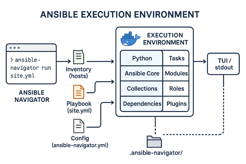 https://github.com/afbjorklund/lima-gui
[Ai ramalama](https://github.com/containers/ramalama)
[Fully Automated Document Management System with Paperless-NGX](https://turalali.com/how-i-built-a-fully-automated-document-management-system-with-paperless-ngx/)
https://oneuptime.com/blog/post/2026-03-04-how-to-deploy-a-spring-boot-application-as-a-systemd-service-on-rhel/view
[example spring boot actuator](https://oneuptime.com/blog/post/2026-01-25-custom-actuator-endpoints-spring-boot/view)
https://github.com/afbjorklund/lima-gui
[Ai ramalama](https://github.com/containers/ramalama)
[Fully Automated Document Management System with Paperless-NGX](https://turalali.com/how-i-built-a-fully-automated-document-management-system-with-paperless-ngx/)
https://oneuptime.com/blog/post/2026-03-04-how-to-deploy-a-spring-boot-application-as-a-systemd-service-on-rhel/view
[example spring boot actuator](https://oneuptime.com/blog/post/2026-01-25-custom-actuator-endpoints-spring-boot/view)
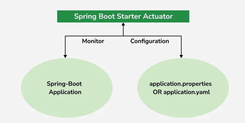 [systemd](https://www.lackhove.de/blog/selfhosting/)
[pikvm](https://pikvm.org/)
[stirling pdf](# stirling pdf)
[stirling config](https://mariushosting.com/how-to-install-stirling-pdf-on-your-ugreen-nas/)
```
podman pull stirlingtools/stirling-pdf:latest
mkdir -p ~/StirlingPDF/{trainingData,extraConfigs,customFiles,logs,pipeline}
podman run -d \
--name stirling-pdf \
-p 8080:8080 \
-v ~/StirlingPDF/trainingData:/usr/share/tessdata \
-v ~/StirlingPDF/extraConfigs:/configs \
-v ~/StirlingPDF/customFiles:/customFiles/ \
-v ~/StirlingPDF/logs:/logs/ \
-v ~/StirlingPDF/pipeline:/pipeline/ \
-e DOCKER_ENABLE_SECURITY=false \
-e LANGS=en_GB \
stirlingtools/stirling-pdf:latest
```
https://ostechnix.com/stirling-pdf-best-open-source-self-hosted-pdf-manipulation-tool/
https://docs.stirlingpdf.com/Installation/Windows%20Installation/
https://github.com/Stirling-Tools/Stirling-PDF/releases/tag/v2.6.0
container_podman_stirling_pdf
================================
version: '3.3'
services:
stirling-pdf:
image: stirlingtools/stirling-pdf:latest
ports:
- '8080:8080'
volumes:
- ~/StirlingPDF/trainingData:/usr/share/tessdata
- ~/StirlingPDF/extraConfigs:/configs
- ~/StirlingPDF/customFiles:/customFiles/
- ~/StirlingPDF/logs:/logs/
- ~/StirlingPDF/pipeline:/pipeline/
environment:
- DOCKER_ENABLE_SECURITY=false
- LANGS=en_GB
https://greenwebpage.com/community/how-to-use-rsync-to-sync-local-and-remote-files-and-directories-in-ubuntu-22-04/
https://sites.ualberta.ca/~clange/Linux/openSUSE/15.6/instructions/openSUSE156_user.html#remote
[zfs, btrfs and e4](https://www.alessioligabue.it/en/blog/btrfs-zfs-ext4-comparison#:~:text=You%20are%20a%20Desktop%2FLaptop,openSUSE)%20use%20it%20by%20default.)
[systemd](https://www.lackhove.de/blog/selfhosting/)
[pikvm](https://pikvm.org/)
[stirling pdf](# stirling pdf)
[stirling config](https://mariushosting.com/how-to-install-stirling-pdf-on-your-ugreen-nas/)
```
podman pull stirlingtools/stirling-pdf:latest
mkdir -p ~/StirlingPDF/{trainingData,extraConfigs,customFiles,logs,pipeline}
podman run -d \
--name stirling-pdf \
-p 8080:8080 \
-v ~/StirlingPDF/trainingData:/usr/share/tessdata \
-v ~/StirlingPDF/extraConfigs:/configs \
-v ~/StirlingPDF/customFiles:/customFiles/ \
-v ~/StirlingPDF/logs:/logs/ \
-v ~/StirlingPDF/pipeline:/pipeline/ \
-e DOCKER_ENABLE_SECURITY=false \
-e LANGS=en_GB \
stirlingtools/stirling-pdf:latest
```
https://ostechnix.com/stirling-pdf-best-open-source-self-hosted-pdf-manipulation-tool/
https://docs.stirlingpdf.com/Installation/Windows%20Installation/
https://github.com/Stirling-Tools/Stirling-PDF/releases/tag/v2.6.0
container_podman_stirling_pdf
================================
version: '3.3'
services:
stirling-pdf:
image: stirlingtools/stirling-pdf:latest
ports:
- '8080:8080'
volumes:
- ~/StirlingPDF/trainingData:/usr/share/tessdata
- ~/StirlingPDF/extraConfigs:/configs
- ~/StirlingPDF/customFiles:/customFiles/
- ~/StirlingPDF/logs:/logs/
- ~/StirlingPDF/pipeline:/pipeline/
environment:
- DOCKER_ENABLE_SECURITY=false
- LANGS=en_GB
https://greenwebpage.com/community/how-to-use-rsync-to-sync-local-and-remote-files-and-directories-in-ubuntu-22-04/
https://sites.ualberta.ca/~clange/Linux/openSUSE/15.6/instructions/openSUSE156_user.html#remote
[zfs, btrfs and e4](https://www.alessioligabue.it/en/blog/btrfs-zfs-ext4-comparison#:~:text=You%20are%20a%20Desktop%2FLaptop,openSUSE)%20use%20it%20by%20default.)
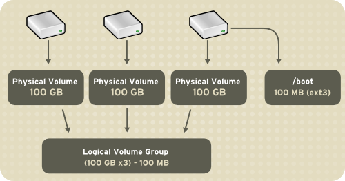 - You are a Desktop/Laptop Linux user: Go with ext4 if you want maximum simplicity and compatibility.
Choose btrfs if you want system snapshots (for easy rollbacks of updates) and compression.
- Many modern distributions (such as Fedora and openSUSE) use it by default.
* You are building a home NAS (e.g. Unraid, Proxmox): This is the btrfs vs. zfs battle.
* Choose ZFS if absolute integrity of your media and backups is priority #1 and you have enough RAM (minimum 8GB+).
* Choose btrfs if you prefer flexibility (e.g., add disks of different sizes) and want a lighter system.
[Promox](https://www.alessioligabue.it/en/blog/install-proxmox)
[proxmox wihout ehernet](https://dev.to/varungujarathi9/setting-up-proxmox-on-a-laptop-without-an-ethernet-port-28n8)
[proxmox -1](https://github.com/retiarylime/proxmox-laptop-wifi)
- You are a Desktop/Laptop Linux user: Go with ext4 if you want maximum simplicity and compatibility.
Choose btrfs if you want system snapshots (for easy rollbacks of updates) and compression.
- Many modern distributions (such as Fedora and openSUSE) use it by default.
* You are building a home NAS (e.g. Unraid, Proxmox): This is the btrfs vs. zfs battle.
* Choose ZFS if absolute integrity of your media and backups is priority #1 and you have enough RAM (minimum 8GB+).
* Choose btrfs if you prefer flexibility (e.g., add disks of different sizes) and want a lighter system.
[Promox](https://www.alessioligabue.it/en/blog/install-proxmox)
[proxmox wihout ehernet](https://dev.to/varungujarathi9/setting-up-proxmox-on-a-laptop-without-an-ethernet-port-28n8)
[proxmox -1](https://github.com/retiarylime/proxmox-laptop-wifi)
 # RAII in rust
https://benjamincongdon.me/blog/2025/12/23/RAII-Guards-and-Newtypes-in-Rust/
# [Money Laundering](https://www.ingenique.net/anti-money-laundering-whitepapers/)
- Dasseti
# [Dynamic array c - stb_ds.h or vector.h](https://lazarusoverlook.com/posts/vector-c-library/)
[stb_ds.h](https://nothings.org/stb_ds/) is a public-domain, single-header-file C library that provides high-performance, cache-friendly data structures like dynamic arrays and hash tables.
The library itself does not manage a general-purpose "cache" in the sense of a CPU cache (e.g., an LRU cache) but its design leverages principles like data locality
to perform efficiently with modern CPU caching.
[hashtable map](https://hackmd.io/q9KOSSvlRUG0w9APyqBgEw)
[video on hashtable](https://www.youtube.com/watch?v=ncHmEUmJZf4)
[hashtable 1](https://codecapsule.com/2013/05/13/implementing-a-key-value-store-part-5-hash-table-implementations/)
[hashtale 2](https://attractivechaos.wordpress.com/2018/10/01/advanced-techniques-to-implement-fast-hash-tables/)
```
#define STB_DS_IMPLEMENTATION
#include "stb_ds.h"
#include
# RAII in rust
https://benjamincongdon.me/blog/2025/12/23/RAII-Guards-and-Newtypes-in-Rust/
# [Money Laundering](https://www.ingenique.net/anti-money-laundering-whitepapers/)
- Dasseti
# [Dynamic array c - stb_ds.h or vector.h](https://lazarusoverlook.com/posts/vector-c-library/)
[stb_ds.h](https://nothings.org/stb_ds/) is a public-domain, single-header-file C library that provides high-performance, cache-friendly data structures like dynamic arrays and hash tables.
The library itself does not manage a general-purpose "cache" in the sense of a CPU cache (e.g., an LRU cache) but its design leverages principles like data locality
to perform efficiently with modern CPU caching.
[hashtable map](https://hackmd.io/q9KOSSvlRUG0w9APyqBgEw)
[video on hashtable](https://www.youtube.com/watch?v=ncHmEUmJZf4)
[hashtable 1](https://codecapsule.com/2013/05/13/implementing-a-key-value-store-part-5-hash-table-implementations/)
[hashtale 2](https://attractivechaos.wordpress.com/2018/10/01/advanced-techniques-to-implement-fast-hash-tables/)
```
#define STB_DS_IMPLEMENTATION
#include "stb_ds.h"
#include 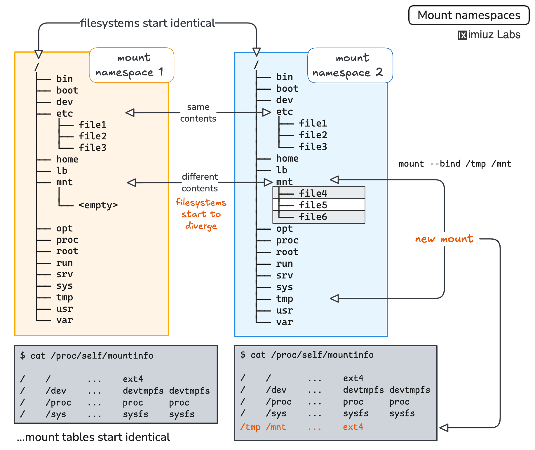
 [unshare namespace run in unix](https://linuxconcept.com/commands/unshare)
Benefits of Using unshare and Namespaces
Process Isolation: Able to run processes independently, preventing interference and providing security.
Resource Management: Efficiently manage and allocate resources without affecting the global environment.
Testing and Development: Create isolated test environments for development and testing purposes without needing full virtual machines.
```
https://dev.to/ajinkya_singh_2c02bd40423/mount-namespace-practice-guide-4c84
unshare -rn
sudo unshare --net bash
sudo unshare --mount bash
sudo lsns
```
|Command |Description|
|---------|-----------|
|podman images -f dangling=true |List dangling images|
|podman image prune -f |Remove only dangling images|
|podman image prune -a -f |Remove all unused images|
|podman container prune -f |Remove stopped containers|
|podman tag localhost/my-image-old:latest localhost/my-image-new:v1| rename tag|
|podman build --rm -t my-image .| remove all the dangling images after build|
Automatically Remove Dangling Images After Build
If you're building images and want to prevent dangling layers, add --rm when building:
podman build --rm -t my-image .
16 xbps-query -f webkit2gtk41-devel | grep javascriptcore
17 pnpm tauri dev
18 ENV PKG_CONFIG_PATH=/usr/lib/pkgconfig:/usr/share/pkgconfig:/usr/local/lib/pkgconfig
19 xbps-install -S webkit2gtk-devel pkg-config
20 xbps-install -S webkit2gtk4-devel pkg-config
21 xbps-install -S void-repo-nonfree void-repo-multilib void-repo-multilib-nonfree
22 pkg-config --modversion webkit2gtk-4.0 # For GTK4
23 export PKG_CONFIG_PATH=/usr/lib/pkgconfig
24 pkg-config --modversion webkit2gtk-4.0 # For GTK4
25 xbps-query -l | grep gtk+3-devel
26 find /usr -name "gdk-3.0.pc"
27 export PKG_CONFIG_PATH=/usr/lib/pkgconfig
28 pkg-config --modversion gdk-3.0
29 sudo xbps-install -S atk-devel cairo-devel pango-devel gdk-pixbuf-devel
30 xbps-install -S atk-devel cairo-devel pango-devel gdk-pixbuf-devel
31 historypwd
To migrate Podman images to another hard drive, you can either permanently change the storage location or create portable copies of your images. Here are the most common and reliable methods.
🔄 Method 1: Permanently Relocate Storage (Change graphRoot)
This method changes the directory where Podman stores all images and containers. It's best if the new hard drive will be the primary storage location.
Step-by-step guide:
1. Find your current storage path with podman info | grep graphRoot .
2. Save all images from the current location to archive files using podman save .
3. Stop and remove all containers and images from Podman's management .
4. Change the configuration to point to the new location on your hard drive by editing the storage configuration file (e.g., ~/.config/containers/storage.conf for a user) and setting the graphroot option to the new path .
5. Reload the images from the archives you saved using podman load .
Best for: Making a new hard drive the default, permanent location for all Podman data.
📦 Method 2: Create Portable Image Archives (Save/Load)
This method creates standalone .tar files of your images, which you can copy anywhere.
How to do it:
· Save an image: podman save -o myimage.tar IMAGE_NAME_OR_ID . You can save multiple images to one file.
· Load an image: podman load -i myimage.tar .
Best for: Creating backups, transferring images to offline machines, or sharing images .
🌐 Method 3: Transfer Between Hosts (podman image scp)
This command uses SSH to copy images directly between two systems. It works even if the destination is a different user account on the same machine .
Example commands:
· Copy to a remote host: podman image scp myimage username@remote_host:: .
· Copy between users locally: podman image scp myimage otheruser@localhost:: .
Best for: Quickly copying images over a network without creating intermediate files, especially between different user accounts .
⚙️ Method 4: Extract Image Contents for File Access
If you need direct access to the files inside an image (like the root filesystem), you can extract them to a directory.
One method is to:
1. Create a temporary container: podman create --name temp_container IMAGE_NAME.
2. Export its filesystem: podman export temp_container | tar -x -C /path/on/new/drive .
3. Remove the container: podman rm temp_container.
Best for: Inspecting or using an image's file contents outside of a container.
💡 Key Considerations
· Manage Data Separately: These methods primarily move the image layers. For persistent data (like databases), remember to separately backup and migrate any volumes or bind mounts used by your containers .
· Check Compatibility: When loading or transferring images between different Podman versions or systems, ensure compatibility to avoid errors .
📝 Summary of Methods
To choose a method, consider your goal:
· Make a new hard drive the main storage: Use Method 1.
· Create a backup or offline copy: Use Method 2.
· Copy an image to another computer quickly: Use Method 3.
· Get the files inside an image: Use Method 4.
If you know which specific method best fits your task or need help with a particular step (like editing the storage.conf file), let me know and I can provide more detailed instructions.
# Dioxus
[pass paramete on rsx!](https://users.rust-lang.org/t/understanding-dioxus-signals-or-state-management-in-general/111611/4)
Seaweed Processing Factory
This food brings many health benefits such as supporting
* thyroid function,
* digestive function and
* reducing the risk of cancer,
* diabetes,
* cardiovascular disease, etc.
In addition, seaweed has the ability to speed up wound recovery. Effective brand and a reasonable choice for the menu of people after surgery.
Postpartum women often eat seaweed to restore health.
Currently, more than 90% of seaweed consumed in Korea comes from seaweed farms. Because natural production is decreasing, seaweed farms
have provided large quantities to serve consumer demand.
# [container guide](https://documentation.suse.com/container/all/html/Container-guide/index.html)
1. sudo systemctl start containerbuild-regionsrv
2. sudo systemctl enable containerbuild-regionsrv
3. podman build --network host build-directory/
FROM registry.suse.com/suse/sle15
RUN zypper ref && zypper --non-interactive in example
ENV BACKUP=/backup
RUN mkdir -p $BACKUP
COPY configuration_example /etc/example/
ENTRYPOINT ["/etc/bin/example"]
[openBSD vs FreeBSD malloc for securiy](https://conclusive.tech/glossary/freebsd-vs-openbsd-which-is-right-for-you/)
[unshare namespace run in unix](https://linuxconcept.com/commands/unshare)
Benefits of Using unshare and Namespaces
Process Isolation: Able to run processes independently, preventing interference and providing security.
Resource Management: Efficiently manage and allocate resources without affecting the global environment.
Testing and Development: Create isolated test environments for development and testing purposes without needing full virtual machines.
```
https://dev.to/ajinkya_singh_2c02bd40423/mount-namespace-practice-guide-4c84
unshare -rn
sudo unshare --net bash
sudo unshare --mount bash
sudo lsns
```
|Command |Description|
|---------|-----------|
|podman images -f dangling=true |List dangling images|
|podman image prune -f |Remove only dangling images|
|podman image prune -a -f |Remove all unused images|
|podman container prune -f |Remove stopped containers|
|podman tag localhost/my-image-old:latest localhost/my-image-new:v1| rename tag|
|podman build --rm -t my-image .| remove all the dangling images after build|
Automatically Remove Dangling Images After Build
If you're building images and want to prevent dangling layers, add --rm when building:
podman build --rm -t my-image .
16 xbps-query -f webkit2gtk41-devel | grep javascriptcore
17 pnpm tauri dev
18 ENV PKG_CONFIG_PATH=/usr/lib/pkgconfig:/usr/share/pkgconfig:/usr/local/lib/pkgconfig
19 xbps-install -S webkit2gtk-devel pkg-config
20 xbps-install -S webkit2gtk4-devel pkg-config
21 xbps-install -S void-repo-nonfree void-repo-multilib void-repo-multilib-nonfree
22 pkg-config --modversion webkit2gtk-4.0 # For GTK4
23 export PKG_CONFIG_PATH=/usr/lib/pkgconfig
24 pkg-config --modversion webkit2gtk-4.0 # For GTK4
25 xbps-query -l | grep gtk+3-devel
26 find /usr -name "gdk-3.0.pc"
27 export PKG_CONFIG_PATH=/usr/lib/pkgconfig
28 pkg-config --modversion gdk-3.0
29 sudo xbps-install -S atk-devel cairo-devel pango-devel gdk-pixbuf-devel
30 xbps-install -S atk-devel cairo-devel pango-devel gdk-pixbuf-devel
31 historypwd
To migrate Podman images to another hard drive, you can either permanently change the storage location or create portable copies of your images. Here are the most common and reliable methods.
🔄 Method 1: Permanently Relocate Storage (Change graphRoot)
This method changes the directory where Podman stores all images and containers. It's best if the new hard drive will be the primary storage location.
Step-by-step guide:
1. Find your current storage path with podman info | grep graphRoot .
2. Save all images from the current location to archive files using podman save .
3. Stop and remove all containers and images from Podman's management .
4. Change the configuration to point to the new location on your hard drive by editing the storage configuration file (e.g., ~/.config/containers/storage.conf for a user) and setting the graphroot option to the new path .
5. Reload the images from the archives you saved using podman load .
Best for: Making a new hard drive the default, permanent location for all Podman data.
📦 Method 2: Create Portable Image Archives (Save/Load)
This method creates standalone .tar files of your images, which you can copy anywhere.
How to do it:
· Save an image: podman save -o myimage.tar IMAGE_NAME_OR_ID . You can save multiple images to one file.
· Load an image: podman load -i myimage.tar .
Best for: Creating backups, transferring images to offline machines, or sharing images .
🌐 Method 3: Transfer Between Hosts (podman image scp)
This command uses SSH to copy images directly between two systems. It works even if the destination is a different user account on the same machine .
Example commands:
· Copy to a remote host: podman image scp myimage username@remote_host:: .
· Copy between users locally: podman image scp myimage otheruser@localhost:: .
Best for: Quickly copying images over a network without creating intermediate files, especially between different user accounts .
⚙️ Method 4: Extract Image Contents for File Access
If you need direct access to the files inside an image (like the root filesystem), you can extract them to a directory.
One method is to:
1. Create a temporary container: podman create --name temp_container IMAGE_NAME.
2. Export its filesystem: podman export temp_container | tar -x -C /path/on/new/drive .
3. Remove the container: podman rm temp_container.
Best for: Inspecting or using an image's file contents outside of a container.
💡 Key Considerations
· Manage Data Separately: These methods primarily move the image layers. For persistent data (like databases), remember to separately backup and migrate any volumes or bind mounts used by your containers .
· Check Compatibility: When loading or transferring images between different Podman versions or systems, ensure compatibility to avoid errors .
📝 Summary of Methods
To choose a method, consider your goal:
· Make a new hard drive the main storage: Use Method 1.
· Create a backup or offline copy: Use Method 2.
· Copy an image to another computer quickly: Use Method 3.
· Get the files inside an image: Use Method 4.
If you know which specific method best fits your task or need help with a particular step (like editing the storage.conf file), let me know and I can provide more detailed instructions.
# Dioxus
[pass paramete on rsx!](https://users.rust-lang.org/t/understanding-dioxus-signals-or-state-management-in-general/111611/4)
Seaweed Processing Factory
This food brings many health benefits such as supporting
* thyroid function,
* digestive function and
* reducing the risk of cancer,
* diabetes,
* cardiovascular disease, etc.
In addition, seaweed has the ability to speed up wound recovery. Effective brand and a reasonable choice for the menu of people after surgery.
Postpartum women often eat seaweed to restore health.
Currently, more than 90% of seaweed consumed in Korea comes from seaweed farms. Because natural production is decreasing, seaweed farms
have provided large quantities to serve consumer demand.
# [container guide](https://documentation.suse.com/container/all/html/Container-guide/index.html)
1. sudo systemctl start containerbuild-regionsrv
2. sudo systemctl enable containerbuild-regionsrv
3. podman build --network host build-directory/
FROM registry.suse.com/suse/sle15
RUN zypper ref && zypper --non-interactive in example
ENV BACKUP=/backup
RUN mkdir -p $BACKUP
COPY configuration_example /etc/example/
ENTRYPOINT ["/etc/bin/example"]
[openBSD vs FreeBSD malloc for securiy](https://conclusive.tech/glossary/freebsd-vs-openbsd-which-is-right-for-you/)

 [Incus](https://blog.hetherington.uk/2025/02/running-unifi-network-application-in-an-incus-container/)
# [Qemu on esp32](https://github.com/AryanBhirud/ESP32_on_QEMU)
[Mock](https://www.throwtheswitch.org/cmock)
[freeRTOS emulation](https://www.freertos.org/Documentation/02-Kernel/03-Supported-devices/04-Demos/03-Emulation-and-simulation/Linux/FreeRTOS-simulator-for-Linux)
https://github.com/esp-rs/esp-wifi.git .
# Or if you need a specific branch:
git clone -b your-branch https://github.com/esp-rs/esp-wifi.git .
```
```
git clone https://github.com/espressif/qemu
brew install libgcrypt
./configure --target-list=xtensa-softmmu \
--enable-gcrypt --enable-debug \
--enable-sanitizers \
--disable-strip --disable-user \
--disable-capstone --disable-vnc \
--disable-sdl --disable-gtk
ninja -C build
```
```
qemu-system-xtensa -nographic -machine esp32 \
-nic user,model=open_eth,
id=lo0,hostfwd=tcp::8000-:80 \
-drive file=merged_qemu.bin,
if=mtd,format=raw
```
```
docker build -t esp\_qemu .
docker run -it --name esp --rm -p 8000:8000 \
-v $(pwd)/build:/app \
esp-qemu:latest qemu-system-xtensa \
-nographic -machine esp32 \
-nic user,model=open\_eth,
id=lo0,hostfwd=tcp::8000-:80 \
-drive file=merged\_qemu.bin,
if=mtd,format=raw
```
[esp32 on qemu](https://techknowhow.club/index.php/2025/08/20/esp32-on-qemu/)
GrapheneOS creates fresh processes (via exec) when spawning applications instead of using the traditional Zygote spawning model.
# C anc CPP ABI
- gcc test_c.c -c
- g++ test_cpp_c.cpp -S
- g++ test_cpp_c.cpp test_c.o
* [c++ plus rust](https://www.encodian.com/blog/create-and-insert-a-document-approval-sheet-using-powerautomate-approval-data/)
* [embedded template c++ Library](https://www.etlcpp.com/releases.html)
* [SAP Ui5 architecture](https://www.tutorialspoint.com/sap_ui5/sap_ui5_architecture.htm)
* [SAp U5 hana](https://sapui5.hana.ondemand.com/sdk/#/topic/28b59ca857044a7890a22aec8cf1fee9)
* [sap ui5 example](https://openui5.org/)
* [sap flori tutorial](https://ui5.sap.com//#/topic/3da5f4be63264db99f2e5b04c5e853db)
* [Flori web design](https://experience.sap.com/fiori-design-web/action-placement/)
* [shell flori tool bar](https://experience.sap.com/fiori-design-web/flexible-column-layout/)
* [sap grid view html](https://experience.sap.com/fiori-design-web/flexible-grid/)
* [Dioxus](https://codesandbox.io/p/github/mattdanielbrown/Dioxus-Example-Projects/master?file=%2Fecommerce-site%2Fsrc%2Fmain.rs%3A19%2C26)
* [Bookmark](https://www.croftsoft.com/library/tutorials/rust-dioxus-project-setup/)
* [docsite dioxus tailwind components](https://github.com/42Angouleme/dioxus-tw-components)
[Coral](https://www.kkp.go.id/storage/Berita/kkp-berhasil-tambah-lagi-2-kawasan-konservasi-laut-PjYn.jpg)rus
rust containers:
struct option
struct Result
## json vs jsonl
## Safe C++
1. A new "safe" context where only a rigorously safe
subset of C++ is allowed
2. Borrow checking to prevent use-after-free bugs
3. Initialization analysis for type safety
4. Pattern matching, choice types, and borrowing
5. Thread-safety features similar to Rust's
send and sync type traits
6. Explicit mutation for references
7. A model for object relocation
Market trends
---
The dried air bladders called fish maws are exported mainly to
* China and Singapore for the manufacture of isinglass, which is used in beverage and cosmetic
industry as well as Chinese traditional medicines (Dutta et al., 2014). The lesser and medium sciaenids are mostly
sold in fresh condition at the local markets or iced and transported to distant interior markets of Odisha, West
- [x] Write the press release
- [ ] Update the website
- [ ] Contact the media
Comparison: Soil pH vs. Water pH & Soil Salinity vs. Brackish Salinity in Mangroves (Indonesia, Lingga Region)
1. Soil pH vs. Water pH in Mangroves
Parameter Soil pH Water pH
Typical Range 6.0–8.5 (slightly acidic to alkaline) 6.5–8.5 (varies with tides)
Influencing Factors - Organic matter decomposition (acidic)
[Incus](https://blog.hetherington.uk/2025/02/running-unifi-network-application-in-an-incus-container/)
# [Qemu on esp32](https://github.com/AryanBhirud/ESP32_on_QEMU)
[Mock](https://www.throwtheswitch.org/cmock)
[freeRTOS emulation](https://www.freertos.org/Documentation/02-Kernel/03-Supported-devices/04-Demos/03-Emulation-and-simulation/Linux/FreeRTOS-simulator-for-Linux)
https://github.com/esp-rs/esp-wifi.git .
# Or if you need a specific branch:
git clone -b your-branch https://github.com/esp-rs/esp-wifi.git .
```
```
git clone https://github.com/espressif/qemu
brew install libgcrypt
./configure --target-list=xtensa-softmmu \
--enable-gcrypt --enable-debug \
--enable-sanitizers \
--disable-strip --disable-user \
--disable-capstone --disable-vnc \
--disable-sdl --disable-gtk
ninja -C build
```
```
qemu-system-xtensa -nographic -machine esp32 \
-nic user,model=open_eth,
id=lo0,hostfwd=tcp::8000-:80 \
-drive file=merged_qemu.bin,
if=mtd,format=raw
```
```
docker build -t esp\_qemu .
docker run -it --name esp --rm -p 8000:8000 \
-v $(pwd)/build:/app \
esp-qemu:latest qemu-system-xtensa \
-nographic -machine esp32 \
-nic user,model=open\_eth,
id=lo0,hostfwd=tcp::8000-:80 \
-drive file=merged\_qemu.bin,
if=mtd,format=raw
```
[esp32 on qemu](https://techknowhow.club/index.php/2025/08/20/esp32-on-qemu/)
GrapheneOS creates fresh processes (via exec) when spawning applications instead of using the traditional Zygote spawning model.
# C anc CPP ABI
- gcc test_c.c -c
- g++ test_cpp_c.cpp -S
- g++ test_cpp_c.cpp test_c.o
* [c++ plus rust](https://www.encodian.com/blog/create-and-insert-a-document-approval-sheet-using-powerautomate-approval-data/)
* [embedded template c++ Library](https://www.etlcpp.com/releases.html)
* [SAP Ui5 architecture](https://www.tutorialspoint.com/sap_ui5/sap_ui5_architecture.htm)
* [SAp U5 hana](https://sapui5.hana.ondemand.com/sdk/#/topic/28b59ca857044a7890a22aec8cf1fee9)
* [sap ui5 example](https://openui5.org/)
* [sap flori tutorial](https://ui5.sap.com//#/topic/3da5f4be63264db99f2e5b04c5e853db)
* [Flori web design](https://experience.sap.com/fiori-design-web/action-placement/)
* [shell flori tool bar](https://experience.sap.com/fiori-design-web/flexible-column-layout/)
* [sap grid view html](https://experience.sap.com/fiori-design-web/flexible-grid/)
* [Dioxus](https://codesandbox.io/p/github/mattdanielbrown/Dioxus-Example-Projects/master?file=%2Fecommerce-site%2Fsrc%2Fmain.rs%3A19%2C26)
* [Bookmark](https://www.croftsoft.com/library/tutorials/rust-dioxus-project-setup/)
* [docsite dioxus tailwind components](https://github.com/42Angouleme/dioxus-tw-components)
[Coral](https://www.kkp.go.id/storage/Berita/kkp-berhasil-tambah-lagi-2-kawasan-konservasi-laut-PjYn.jpg)rus
rust containers:
struct option
struct Result
## json vs jsonl
## Safe C++
1. A new "safe" context where only a rigorously safe
subset of C++ is allowed
2. Borrow checking to prevent use-after-free bugs
3. Initialization analysis for type safety
4. Pattern matching, choice types, and borrowing
5. Thread-safety features similar to Rust's
send and sync type traits
6. Explicit mutation for references
7. A model for object relocation
Market trends
---
The dried air bladders called fish maws are exported mainly to
* China and Singapore for the manufacture of isinglass, which is used in beverage and cosmetic
industry as well as Chinese traditional medicines (Dutta et al., 2014). The lesser and medium sciaenids are mostly
sold in fresh condition at the local markets or iced and transported to distant interior markets of Odisha, West
- [x] Write the press release
- [ ] Update the website
- [ ] Contact the media
Comparison: Soil pH vs. Water pH & Soil Salinity vs. Brackish Salinity in Mangroves (Indonesia, Lingga Region)
1. Soil pH vs. Water pH in Mangroves
Parameter Soil pH Water pH
Typical Range 6.0–8.5 (slightly acidic to alkaline) 6.5–8.5 (varies with tides)
Influencing Factors - Organic matter decomposition (acidic) - Sulfide oxidation (acidic)
- Tidal flushing (neutralizing)
- Mangrove root exudates - Tidal influence (seawater pH ~8.1)
- Freshwater input (lower pH)
- Organic acids from leaf litter Measurement Method - 1:1 soil-water slurry (standard)
- 1:2.5 or saturated paste (more precise) - Direct pH electrode in water sample Expected in Lingga 6.5–7.8 (moderately acidic to neutral due to peat and tidal influence) 7.2–8.2 (brackish influence from Malacca Strait) 2. Soil Salinity vs. Brackish Water Salinity in Mangroves Parameter Soil Salinity Brackish Water Salinity Typical Range 5–30 ppt (hypersaline in dry zones) 5–25 ppt (varies with tides) Influencing Factors - Tidal inundation (salt deposition)
- Evaporation (increases salinity)
- Freshwater seepage (dilutes salt)
- Mangrove salt exclusion (roots filter salt) - Tidal mixing (seawater ~35 ppt + river input)
- Rainfall dilution (monsoon effect)
- Distance from sea (higher upstream) Measurement Method - EC meter (1:5 soil-water extract)
- Saturated paste extract (more accurate) - Salinity refractometer/EC meter
- Lab analysis (chlorinity) Expected in Lingga 10–25 ppt (moderate-high due to tidal influence) 15–25 ppt (brackish, influenced by Malacca Strait & rivers) Key Findings for Lingga Mangroves (Indonesia) pH Dynamics: Soil pH is slightly acidic to neutral (6.5–7.8) due to organic matter and tidal buffering. Water pH is more stable (7.2–8.2) due to seawater influence. Salinity Variations: Soil salinity (10–25 ppt) is influenced by tidal cycles and evaporation. Brackish water (15–25 ppt) reflects a mix of seawater and river inputs. Ecological Implications: Mangrove species (e.g., Rhizophora, Avicennia) adapt to moderate salinity & pH fluctuations. High salinity (>25 ppt) may reduce biodiversity, favoring salt-tolerant species. Recommendations for Study in Lingga Field Measurements: Use pH/EC meters for soil & water samples. Compare dry vs. wet season salinity changes. Lab Analysis: Test soil texture (clay/sand affects salt retention). Analyze porewater salinity for finer gradients. Would you like specific methods for sampling or data analysis in this region? yes Great! Below is a detailed methodology for sampling and analyzing soil pH, water pH, and salinity in the mangrove ecosystems of Lingga, Indonesia, including field and lab techniques. 1. Field Sampling Protocol A. Soil Sampling (for pH & Salinity) Sampling Design: Use stratified random sampling across different zones (seaward, mid, landward). Collect 3–5 replicates per zone for statistical reliability. Depth of Sampling: Surface (0–10 cm) – Most affected by tides & root activity. Subsurface (10–30 cm) – For salt accumulation trends. Tools Required: Stainless steel auger or soil corer. Clean plastic bags (avoid metal/contamination). GPS for location marking. B. Water Sampling (for pH & Salinity) Sampling Points: Tidal creeks (high/low tide). Porewater (from soil pits). Adjacent river/sea (reference). Collection Method: Use sterile bottles (rinsed 3x with sample water). Avoid air bubbles (affects pH). Measure in-situ (pH, EC, temp) with portable meters. 2. Laboratory Analysis A. Soil pH Measurement 1:1 Soil-Water Slurry Method (Standard for Mangroves): Mix 10g dry soil + 10mL distilled water, stir, wait 30 mins. Measure with calibrated pH meter (buffer at 4.01, 7.01, 10.01). Saturated Paste Method (More Precise): Add water until soil glistens, wait 1 hour, extract liquid for pH. B. Soil Salinity (EC – Electrical Conductivity) 1:5 Soil-Water Extract: Mix 20g soil + 100mL distilled water, shake 1 hour, filter. Measure EC (µS/cm) and convert to ppt (≈ EC × 0.64). Saturated Paste Extract (SPE): More accurate for saline soils (measures "real" porewater salinity). C. Water pH & Salinity pH: Use fresh samples (avoid CO₂ absorption). Salinity: Refractometer (direct reading in ppt). EC Meter (convert using EC × 0.47 ≈ ppt for brackish water). 3. Data Analysis & Interpretation A. Statistical Tools Descriptive Stats: Mean ± SD for pH/salinity per zone. ANOVA/T-test: Compare zones/seasons. Correlation: pH vs. salinity, soil vs. water. B. Mapping & Trends GIS/Interpolation: Plot spatial salinity gradients. Seasonal Variation: Compare monsoon vs. dry season. 4. Expected Challenges & Solutions Challenge Solution Tidal access limitations Sample at low tide. Electrode drift in saline water Frequent calibration with KCl buffers. Organic matter interference Use SPE method for salinity. 5. Equipment Checklist ✅ Field: pH/EC meter, refractometer, GPS, auger, sample bottles. ✅ Lab: Analytical balance, shaker, filter papers, calibration buffers. Next Steps for Your Study Pilot Sampling: Test methods in 1–2 sites before full survey. Local Collaboration: Engage with Universitas Riau or LIPI for lab access. Climate Data: Obtain rainfall/tide charts for Lingga. Would you like a sample data sheet template or references for mangrove soil studies in SE Asia?